Recently I’ve been working on the project of training an AI for Doom, which is a classic FPS game. Luckily, the control side API has been provided by the VizDoom team, so the rest of the task is with how to train it.
While I’m not going to get into terribly detailed descriptions here, you are very welcomed to take a look at our presentation poster, and the final project paper (much longer and more details).
Why Doom?
Compared to other games that deep reinforcement learning (DRL) has been focusing on, such as Atari and Pong, Doom is very different:
- Doom is much more complicated. While Atari has only two actions (
MOVE_LEFTandMOVE_RIGHT), Doom has a dozen of actions supported (e.g.MOVE_LEFT,TURN_LEFT,ATTACK,SPEED,SELECT_NEXT_WEAPON, etc.). This increases the inherent dimension within the task. - Doom is a 3D game. Both Atari and Pong are really on one plane, and the concept of distance makes more sense in Doom.
- Doom is more strategic. Atari and Pong certainly involves strategies as well, but it’s more about how to score better. For Doom, the strategy consists not only of actions, but also navigations, and even a sense of self-awareness (for example, if you know your health value is low, you may want to hide).
It is therefore a challenging task to train an AI in games as complicated as Doom.
Prior Works?
Yes, there are a few brilliant prior works. Chaplot and Lample published their results, which can be found here. They primarily used the DRQN (deep recurrent Q-network) and LSTM to do the training. The result of their AI’s performance can be found on the VizDoom website. According to their paper, the eventual AI took more than a week to finish training. Also, they tweaked the API a little bit so that the information about the enemy was available for them to do some pre-training. Impressive work.
Classic Models
So far, the models that perform best are based on Q-learning, including DQN, Double DQN, as well as applying experience replay memory on them (which has the effect of stabilizing the training). Some recent works on prioritized experience replay suggests that by assigning weights to the memories, the training process can be further accelerated. The idea behind Q learning is simple. But before that, we need to know what “reinforcement learning” is trying to learn.
Reinforcement Learning
The reinforcement learning is really about 2 things: reward and action. Personality psychology points out the giving rewards helps shape behavior. Here the idea is the same: through rewards, we can define a loss function, through which we can update our function and thus train the program.
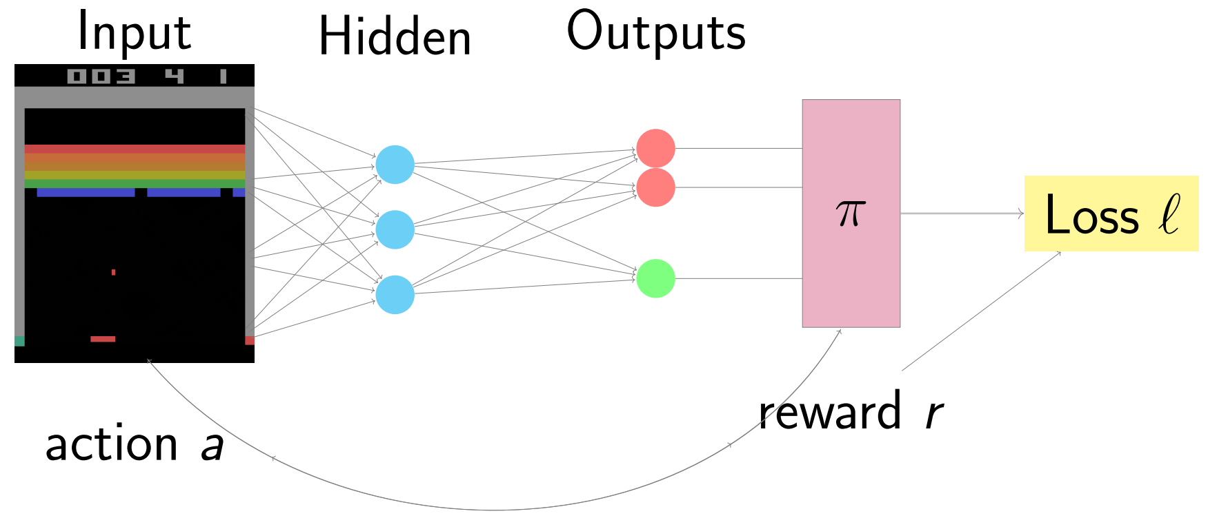
At a certain state \( s_t \), the action \( a_t \) that the agent performs will bring it to the next state, \( s_{t+1} \) and generate an immediate reward \( r_t \). But is this \( r_t \) the true worth of this action? No. An action may generate an outcome that takes some time to show its effect. For example, the benefit of getting an additional armor is not obvious unless you take a hit. Therefore, to get the true value of the pair \( s_t, a_t \), we need to look at the total expected rewards in the future. In RL, this is frequently characterized as the state value function \( V(s) = \mathbb{E}[r_t + \gamma r_{t+1} + \dots] \). That is, given the state \( s \), what is the future discounted total reward that we should expect? Obviously, if we have \( V(s) \), then we can simply choose the action that leads to the best state through our action. We can also train a policy \( \pi (s \vert a) \), which is a probability distribution on the list of suggested actions \( a \) given the current state \( s \). If we have this, then basically we can directly select an action based on the distribution.
So, either having an \( V \) or having a \( \pi \) would be great.
Q-learning
Q-learning has been a popular method to estimate the state value function \( V(s) \) that we mentioned above. In particular, here is the definition of a Q value:
\[Q^\pi(s,a) = \mathbb{E}[R_t | s_t=s, a]\]which can be interpreted as “the expected total future rewards, given that we are at state \( s \), and take action \( a \) next”. If states \( s \) and actions \( a \) are both finite and discrete, then we can actually keep a table that updates the Q values of different state-action pairs. But if the domain is continuous, usually, we use neural networks to approximate the \( Q \) function. Here is how the \( Q \) values get updated, in general:
\[Q(s_t, a_t) \longleftarrow Q(s_t, a_t) + \underbrace{\alpha_t}_{\text{learning rate}} \cdot \big( r_t + \gamma \cdot \underbrace{\max_{a'} Q(s', a')}_{\text{estimate of rewards after} t} - Q(s_t, a_t)\big)\]Why does this make sense? Recall that by how we defined \( Q \), we essentially have \( Q(s’, a’) = \mathbb{E}[r_{t+1} + \gamma r_{t+2} + \gamma^2 r_{t+3} + \dots \vert s_{t+1}=s’, a’]\). So by linearity of expectation, we have
\[\begin{aligned} \mathbb{E}_t[R_t | s_t=s, a] &= \mathbb{E}_t[r_t + \gamma r_{t+1} + \gamma^2 r_{t+2} + \dots] \\ &= r_t + \gamma \cdot \mathbb{E}_t[r_{t+1} + \gamma r_{t+2} + \dots] = r_t + \gamma \cdot \max_{a'} Q(s', a') \end{aligned}\]Keep updating the \( Q \) function in the manner defined above, that is the essence of the Q-learning.
A3C Model
Q-learning based methods have two major shortcomings: (1) to stablize the training, replay memory is often needed. Storing lots of past experience can quickly consume the memory in your computer. (2) Q-learning, which takes the max among the next state’s possible actions, is off-policy (i.e. it has no policy to rely on!). This limits the scope of the algorithms that Q-learning can work on.
A latest solution proposed as an alternative is A3C, which stands for A(synchronous) A(dvantage) A(ctor)-C(ritic) model. This was brought up by Minh et al. at Google DeepMind in Summer 2016 (see paper here).
Advantage Actor-Critic Part
One major difference between Q-learning methods and A3C is that, while Q-learning tries to use the \( Q \) function to estimate \( V \), A3C model tries to study both \( V \) and \( \pi \) functions simultaneously. How does it accomplish that? Look at the figure below:
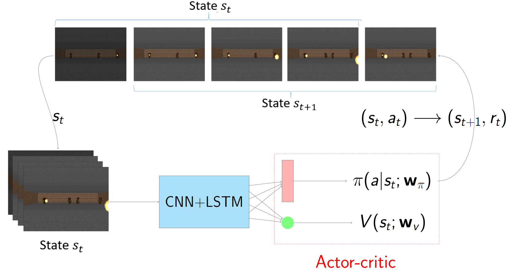
Whereas CNN and LSTM are still used in the similar way as before to extract features out of the state (which is a stack of the frames), the real power of A3C comes after: the network splits into two sub-networks, one approximating the \( \pi \) function (which is a distribution, so we use softmax) another approximating \( V \) function (which is a single value). Then, since we have the policy function, we can choose the action at time \( t \), namely \( a_t \) so as to generate the next state as well as the reward:
\[(s_t, a_t) \longrightarrow (s_{t+1}, r_t)\]Repeating the process for some \( t_{\text{max}} \) times (a hyperparameter that defines how long is a training step), we should be able to collect a bunch of rewards starting from time \( t \): \( r_t, r_{t+1}, r_{t+2}, \dots \). We can now define the “real future reward at time \( t \)” as:
\[R_t = r_t + \gamma r_{t+1} + \gamma^2 r_{t+2} + \dots + \gamma^{t_\text{max}-1} r_{t+t_{\text{max}}-1} + \gamma^{t_{\text{max}}} V(s_{t+t_{\text{max}}})\]Why do we have a \( V \) at the end? Well, recall that \( V(s_T) \) represents the future reward starting from time \( T \). Here estimate the reward after \( t + t_{\text{max}} \) using \( V \).
What next? Minh et al. used the advantage function as the key component to define a loss and a score function. In particular, let
\[A(s_t, a_t, \mathbf{w}_\pi, \mathbf{w}_V) = R_t - V(s_t)\]which we can understand as “how much does the real reward that we get outperforms our expected reward?” Of course, we want to go beyond the expectation as much as possible (i.e. our advantage margin). Thus we define the score and loss functions:
\[\begin{aligned} K_\pi^t &= \log(\pi(a_t \vert s_t; \mathbf{w}_\pi)) \cdot \underbrace{(R_t - V(s_t))}_{\text{Advantage}} + \beta \cdot \underbrace{H(\pi)}_{\text{entropy loss}} \\ L_V^t &= (R_t - V(s_t))^2 \end{aligned}\]Value \( K \) here represents the score, which is what we want to maximize. The log term was on the action that we chose. Since log is monotone, this can be understood as our objective to choose the action just chosed with probability as high as possible. The entropy loss added, \( \beta H(\pi) \), means we don’t want the policy distribution to be simply uniform— which is no different from choosing an action randomly. Meanwhile, the loss function is a lot easier to understand: we want to train the \( V \) network so that its estimate of the future reward is as close to the real reward \( R_t \) as possible.
In summary, when updating the \( \pi \) and \( V \) networks (which share a common portion, the CNN+LSTM part!), we can simply do
\[\begin{aligned} \mathbf{w}_\pi &\longleftarrow \mathbf{w}_\pi + \alpha \cdot \nabla_{\mathbf{w}_\pi} K_\pi^t \\ \mathbf{w}_V & \longleftarrow \mathbf{w}_V - \alpha \cdot \nabla_{\mathbf{w}_V} L_V^t \end{aligned}\]Note that we want to maximize \( K \), so we do gradient ascent; while to minimize \( L \), we take gradient descent. In implementation, we used RMSProp.
Asynchronous Part
Another very important aspect of the A3C model is the async nature of this algorithm, which helps it avoid some critical problems in Q-learning based techniques. In particular, one classic problem that Q-learning based methods has is that it is highly subject to time bias. For instance, the situation an agent encounters from time \( t=2s \) to \( t=6s \) may be extremely similar. To solve this problem, methods like DQN also added the prioritized replay memory, which was proposed and used in many DRL projects recently.
What is the replay memory? Well, basically, you gather around all the experiences you had, in the form of batches of frames. Then, when a new situation (i.e. a new frame) comes in, you not only look at the new frame, but also randomly pick an old frame— in other words, the agent is able to remember and reuse experiences from the past. As Schaul et al. introduced in their famous Prioritized Experience Replay paper, this is able to boost the DQN performance by a significant amount.
However, A3C solves this problem in another way. Essentially, having multiple agents each exploring a different situation, the updates on the globally shared neural network balances itself— just like how replay memory picks out the past experience to balance the training, except that the balance now comes from right now.
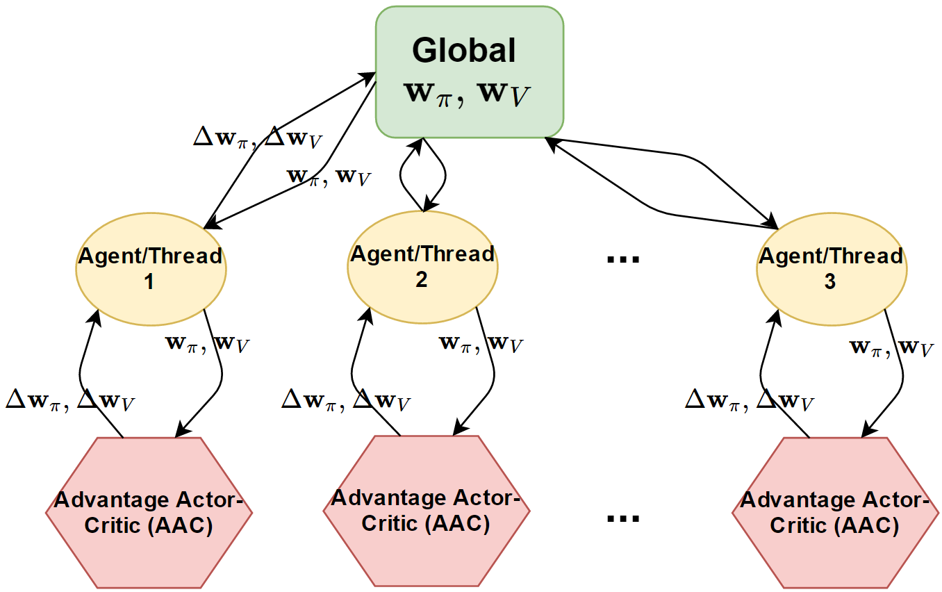
The asynchronous part of this model essentially works as follows (you can also find the details in our project final paper, which is now available!):
And here is a demo of what “asynchronous agents exploring the map” looks like:
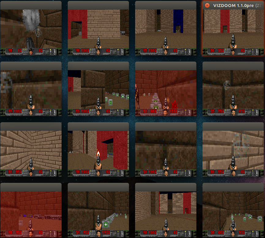
Each thread (i.e. agent) essentially run for some time $T$. Then, it collects the rewards it receives during these time, discounts them by “interest rate” \( \gamma \), and use this to compute the score & loss that are needed for the gradient updates. These updates are then flushed back to a globally shared network. Nevertheless, this global NN does not represent the brain of any particular agents. When the agent finishes send the updates to the global NN, it synchronizes with this global NN so that not only its own updates but also updates from other agents are now learned.
More?
Certainly, the A3C model is at the core of our design of this cool AI. But meanwhile, the project is much more complex than simply this model. For instance, how do we best categorize the datasets that we use (visualizations, game variables, etc.) and harness their power more efficiently? How did we test our AI and what did we accomplish? What were some limitations? What other methods are possible for the improvements? While this post serves primarily as an introduction to this project and the method we use, I hope you can find more fun by reading our final project paper over here.